matlab-with-python-book
5. Call Python AI libraries from MATLAB
In this Chapter we will look at different Python libraries for Artificial Intelligence, both Machine Learning & Deep Learning (like Scikit-learn and TensorFlow) and how to call them from MATLAB.
Those steps can be integrated in a typical AI workflow:

5.1. Call Scikit-learn from MATLAB
The Iris flower dataset is a multivariate data set introduced by the British statistician and biologist Ronald Fisher. This data set consists of 3 different types of irises’ (Setosa, Versicolour, and Virginica) petal and sepal length, stored in a 150x4 numpy.ndarray. The rows being the samples and the columns being: Sepal Length, Sepal Width, Petal Length and Petal Width.
Setup on MATLAB Online to retrieve and install the necessary Python packages:
% Check if we are running on MATLAB Online
if ~isDesktop
    setuppip
    pkg = "scikit-learn pandas pyarrow";
    pipinstall(pkg)
    pipshow(pkg)
end
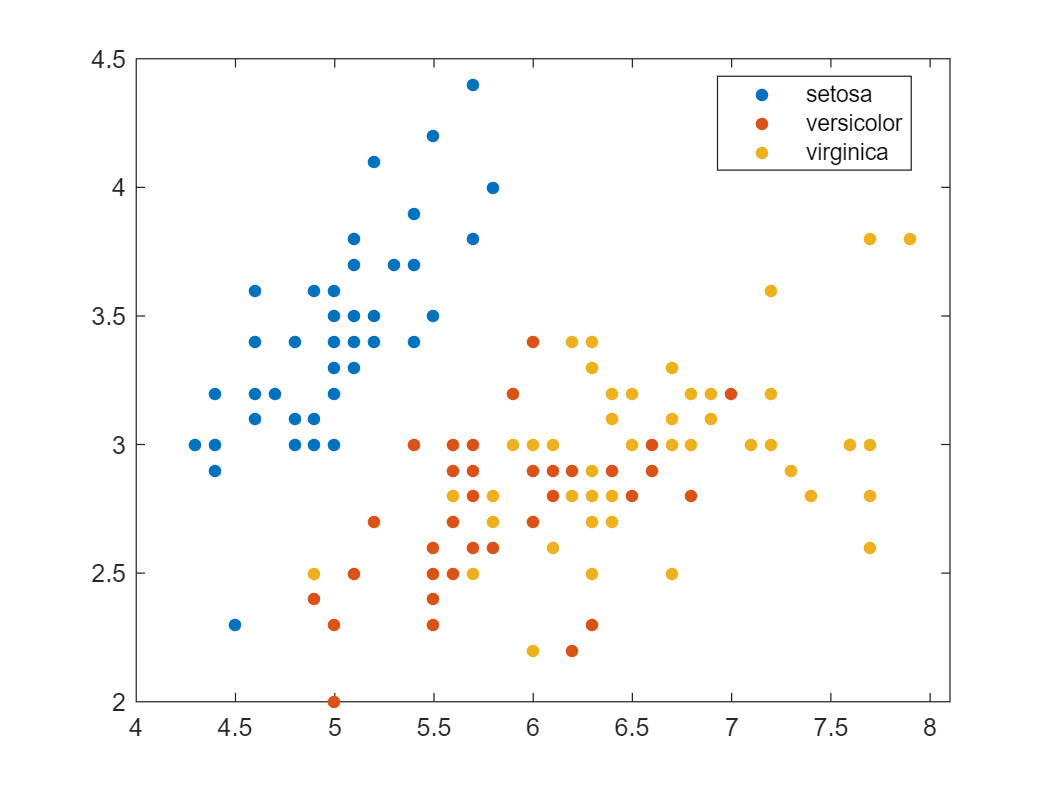
You can also find this dataset in MATLAB, as it is shipped with a list of Sample Data Sets as part of the Stats \& Machine Learning Toolbox:
load fisheriris.mat
gscatter(meas(:,1),meas(:,2),species)
Or retrieve the dataset from the Scikit-learn library (inside of MATLAB still):
iris_dataset = py.sklearn.datasets.load_iris()
iris_dataset =
  Python Bunch with no properties.

    {'data': array([[5.1, 3.5, 1.4, 0.2],
           [4.9, 3. , 1.4, 0.2],
           [4.7, 3.2, 1.3, 0.2],
           [4.6, 3.1, 1.5, 0.2],
           [5. , 3.6, 1.4, 0.2],
           [5.4, 3.9, 1.7, 0.4],
            ...
           [6.2, 3.4, 5.4, 2.3],
           [5.9, 3. , 5.1, 1.8]]),
           'target': array([0, 0, 0, 0, 0, 0, 0, 0, 0, 0, 0, 0, 0, 0, 0, 0, 0, 0, 0, 0, 0, 0,
           0, 0, 0, 0, 0, 0, 0, 0, 0, 0, 0, 0, 0, 0, 0, 0, 0, 0, 0, 0, 0, 0,
           0, 0, 0, 0, 0, 0, 1, 1, 1, 1, 1, 1, 1, 1, 1, 1, 1, 1, 1, 1, 1, 1,
           1, 1, 1, 1, 1, 1, 1, 1, 1, 1, 1, 1, 1, 1, 1, 1, 1, 1, 1, 1, 1, 1,
           1, 1, 1, 1, 1, 1, 1, 1, 1, 1, 1, 1, 2, 2, 2, 2, 2, 2, 2, 2, 2, 2,
           2, 2, 2, 2, 2, 2, 2, 2, 2, 2, 2, 2, 2, 2, 2, 2, 2, 2, 2, 2, 2, 2,
           2, 2, 2, 2, 2, 2, 2, 2, 2, 2, 2, 2, 2, 2, 2, 2, 2, 2]), 'frame': None, 'target_names': array(['setosa', 'versicolor', 'virginica'], dtype='<U10'), 'DESCR': '...', 'feature_names': ['sepal length (cm)', 'sepal width (cm)', 'petal length (cm)', 'petal width (cm)'], 'filename': 'iris.csv', 'data_module': 'sklearn.datasets.data'}
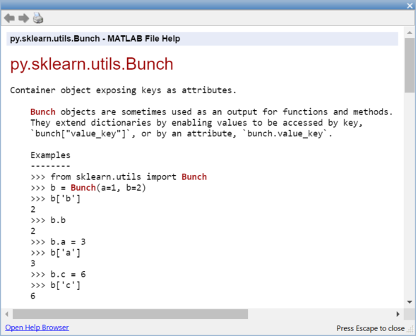
Scikit-learn datasets are returned as a Bunch object. You can access the Python modules documentation directly from within MATLAB:
This dataset can be passed to MATLAB as a struct:
struct(iris_dataset)
ans =
             data: [1x1 py.numpy.ndarray]
           target: [1x1 py.numpy.ndarray]
            frame: [1x1 py.NoneType]
     target_names: [1x1 py.numpy.ndarray]
            DESCR: [1x2782 py.str]
    feature_names: [1x4 py.list]
         filename: [1x8 py.str]
      data_module: [1x21 py.str]
X_np = iris_dataset{'data'}
X_np =
  Python ndarray:

    5.1000    3.5000    1.4000    0.2000
    4.9000    3.0000    1.4000    0.2000
    4.7000    3.2000    1.3000    0.2000
    4.6000    3.1000    1.5000    0.2000
    ...
    5.9000    3.0000    5.1000    1.8000

    Use details function to view the properties of the Python object.

    Use double function to convert to a MATLAB array.
X_ml = double(X_np)
X_ml = 150x4
    5.1000    3.5000    1.4000    0.2000
    4.9000    3.0000    1.4000    0.2000
    4.7000    3.2000    1.3000    0.2000
    4.6000    3.1000    1.5000    0.2000
    5.0000    3.6000    1.4000    0.2000
    5.4000    3.9000    1.7000    0.4000
    4.6000    3.4000    1.4000    0.3000
    5.0000    3.4000    1.5000    0.2000
    4.4000    2.9000    1.4000    0.2000
    4.9000    3.1000    1.5000    0.1000
X = X_ml(:,1:2)
X = 150x2
    5.1000    3.5000
    4.9000    3.0000
    4.7000    3.2000
    4.6000    3.1000
    5.0000    3.6000
    5.4000    3.9000
    4.6000    3.4000
    5.0000    3.4000
    4.4000    2.9000
    4.9000    3.1000
y = iris_dataset{'target'}
y =
  Python ndarray:

   0   0   0   0   0   0   0   0   0   0   0   0   0   0   0   0   0   0   0   0   0   0   0   0   0   0   0   0   0   0   0   0   0   0   0   0   0   0   0   0   0   0   0   0   0   0   0   0   0   0   1   1   1   1   1   1   1   1   1   1   1   1   1   1   1   1   1   1   1   1   1   1   1   1   1   1   1   1   1   1   1   1   1   1   1   1   1   1   1   1   1   1   1   1   1   1   1   1   1   1   2   2   2   2   2   2   2   2   2   2   2   2   2   2   2   2   2   2   2   2   2   2   2   2   2   2   2   2   2   2   2   2   2   2   2   2   2   2   2   2   2   2   2   2   2   2   2   2   2   2

    Use details function to view the properties of the Python object.

    Use int64 function to convert to a MATLAB array.
% y_ml = int64(y)
We won’t translate the Python ndarray into a MATLAB datatype just yet, as we will use a cool feature of Python to translate the list of ordinal values into a list of categorical species. Those features can be leveraged in MATLAB with a few calls to pyrun
pyrun('dict = {0: "setosa",1: "versicolor", 2: "virginica"}')
s = pyrun('species = [dict[i] for i in y]','species',y = y) % pass y as input, and retrieve species as output
s =
  Python list with values:

    ['setosa', 'setosa', 'setosa', 'setosa',
    ...
    'versicolor', 'versicolor', 'versicolor',
    ...
    'virginica', 'virginica', 'virginica']

    Use string, double or cell function to convert to a MATLAB array.
Finally, you can retrieve the Python list as a MATLAB categorical variable:
s = string(s);
species = categorical(s)
species = 1x150 categorical
setosa       setosa       setosa       setosa       setosa       setosa       setosa       setosa       setosa       setosa       setosa       setosa       setosa       setosa       setosa       setosa       setosa       setosa       setosa       setosa       setosa       setosa       setosa       setosa       setosa       setosa       setosa       setosa       setosa       setosa
Another approach for the preprocessing in Python can be performed with pyrunfile
[X,y,species] = pyrunfile('iris_data.py',{'Xl','y','species'})
X =
  Python list with values:

    [[5.1, 3.5], [4.9, 3.0],
    ... [5.9, 3.0]]

    Use string, double or cell function to convert to a MATLAB array.

y =
  Python ndarray:

   0   0   0   0   0   0   0   0   0   0   0   0   0   0   0   0   0   0   0   0   0   0   0   0   0   0   0   0   0   0   0   0   0   0   0   0   0   0   0   0   0   0   0   0   0   0   0   0   0   0   1   1   1   1   1   1   1   1   1   1   1   1   1   1   1   1   1   1   1   1   1   1   1   1   1   1   1   1   1   1   1   1   1   1   1   1   1   1   1   1   1   1   1   1   1   1   1   1   1   1   2   2   2   2   2   2   2   2   2   2   2   2   2   2   2   2   2   2   2   2   2   2   2   2   2   2   2   2   2   2   2   2   2   2   2   2   2   2   2   2   2   2   2   2   2   2   2   2   2   2

    Use details function to view the properties of the Python object.

    Use int64 function to convert to a MATLAB array.

species =
  Python list with values:

    ['setosa', 'setosa', 'setosa', 'setosa',
    ...
    'versicolor', 'versicolor', 'versicolor',
    ...
    'virginica', 'virginica', 'virginica']

    Use string, double or cell function to convert to a MATLAB array.
This is what the python scripts looks like:
iris_data.py
from sklearn import datasets
iris = datasets.load_iris()

X = iris.data[:, :2]  # we only take the first two features (sepal)
Xl = X.tolist()
y = iris.target
dict = {0: "setosa", 1: "versicolor", 2: "virginica"}
species = [dict[i] for i in y]
In this case, we are retrieving a list of lists, instead of a Numpy array. This will require some manual data marshalling:
Xc = cell(X)'
| |1| |:–:|:–:| |1|1x2 list| |2|1x2 list| |3|1x2 list| |4|1x2 list| |5|1x2 list| …
Xc1 = cell(Xc{1})
| 1 | 2 | |
|---|---|---|
| 1 | 5.1000 | 3.5000 |
cell2mat(Xc1)
ans = 1x2
    5.1000    3.5000
The previous steps are included in the helper function dataprep (at the end of the live script):
function Xp = dataprep(X)
  Xc = cell(X)';
  Xcc = cellfun(@cell,Xc,'UniformOutput',false);
  Xcm = cellfun(@cell2mat,Xcc,'UniformOutput',false);
  Xp = cell2mat(Xcm);
end
X_ml = dataprep(X);
y_ml = double(y);
s = string(species);
species = categorical(s);
Another approach that doesn’t involve data transfer is to perform the preprocessing in Python and save the results as Parquet file
pyrunfile('iris_data_save.py')
Then, load the Parquet file in MATLAB directly as table
T = parquetread("iris.parquet")
| lenght | width | species | |
|---|---|---|---|
| 1 | 5.1000 | 3.5000 | “setosa” |
| 2 | 4.9000 | 3 | “setosa” |
| 3 | 4.7000 | 3.2000 | “setosa” |
| 4 | 4.6000 | 3.1000 | “setosa” |
| 5 | 5 | 3.6000 | “setosa” |
| 6 | 5.4000 | 3.9000 | “setosa” |
| 7 | 4.6000 | 3.4000 | “setosa” |
| 8 | 5 | 3.4000 | “setosa” |
| 9 | 4.4000 | 2.9000 | “setosa” |
| 10 | 4.9000 | 3.1000 | “setosa” |
| 11 | 5.4000 | 3.7000 | “setosa” |
| 12 | 4.8000 | 3.4000 | “setosa” |
| 13 | 4.8000 | 3 | “setosa” |
| 14 | 4.3000 | 3 | “setosa” |
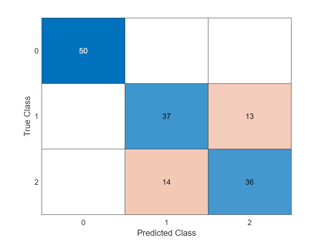
Call the Scikit-Learn Logistic Regression and its fit and predict methods directly:
model = py.sklearn.linear_model.LogisticRegression();
model = model.fit(X,y); % pass by object reference
y2 = model.predict(X);
y2_ml = double(y2);
confusionchart(y_ml,y2_ml)
Call the Scikit-Learn model through a wrapper module:
model = py.iris_model.train(X,y);
y2 = py.iris_model.predict(model, X)
y2 =
  Python ndarray:

   0   0   0   0   0   0   0   0   0   0   0   0   0   0   0   0   0   0   0   0   0   0   0   0   0   0   0   0   0   0   0   0   0   0   0   0   0   0   0   0   0   0   0   0   0   0   0   0   0   0   2   2   2   1   2   1   2   1   2   1   1   1   1   1   1   2   1   1   1   1   1   1   1   1   2   2   2   2   1   1   1   1   1   1   1   2   2   1   1   1   1   1   1   1   1   1   1   1   1   1   2   1   2   2   2   2   1   2   2   2   2   2   2   1   1   2   2   2   2   1   2   1   2   1   2   2   1   1   2   2   2   2   2   2   1   2   2   2   1   2   2   2   1   2   2   2   1   2   2   1

    Use details function to view the properties of the Python object.

    Use int64 function to convert to a MATLAB array.
Precision of the model based on the training set:
sum(y_ml == y2)/length(y_ml)
ans = 0.8200
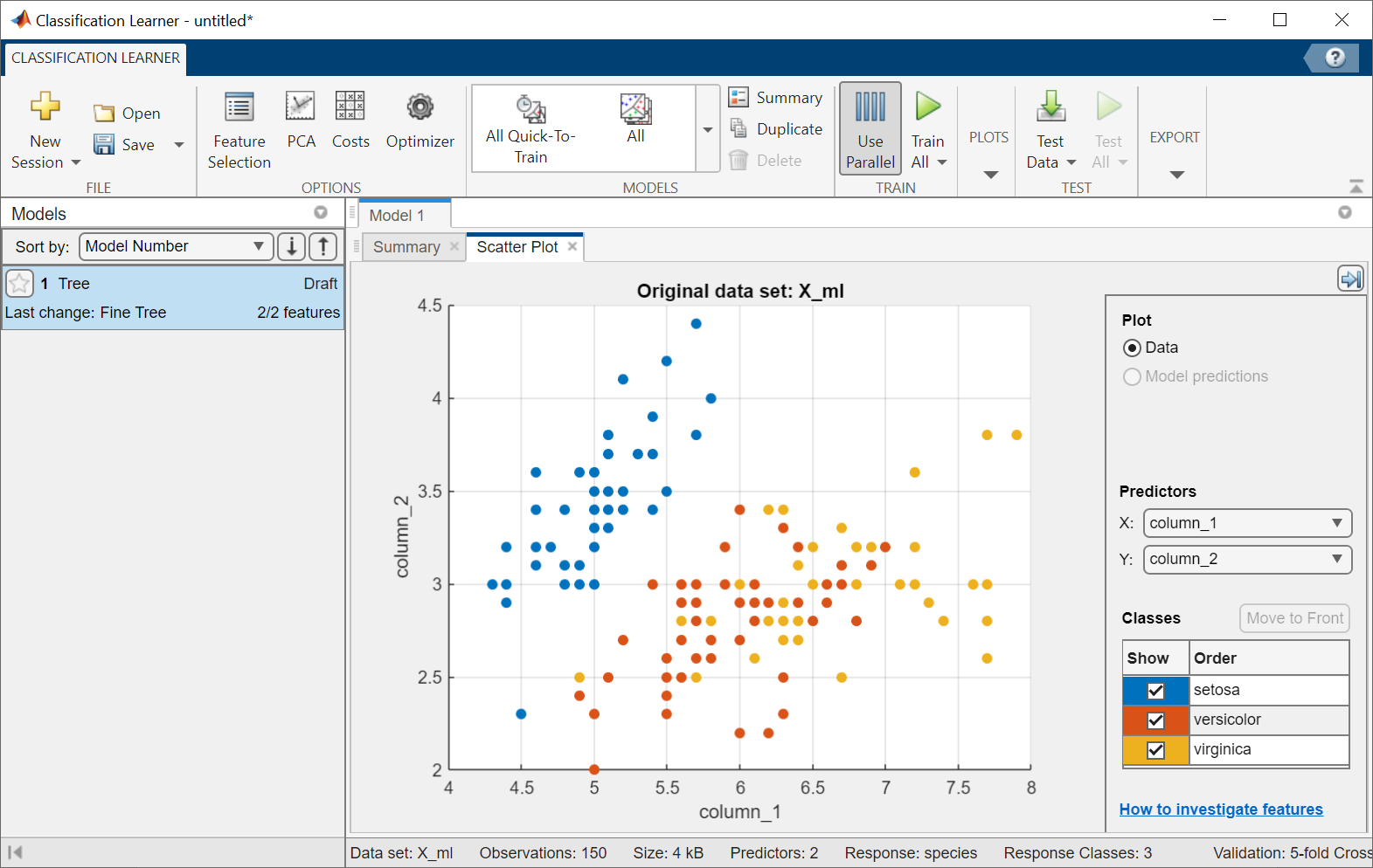
Alternatively, you can train all sorts of classification models in MATLAB. If you don’t feel too comfortable with the various machine learning methods, you can simply try out the results from different types of models with an app:
classificationLearner(X_ml,species)
5.2. Call TensorFlow from MATLAB
Let’s introduce the use of Tensorflow with the getting started tutorial:
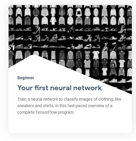
This guide uses the Fashion MNIST dataset which contains 70,000 grayscale images in 10 categories.
The images show individual articles of clothing at low resolution (28 by 28 pixels).
This example is curated by Zalando, under a MIT License.
First let’s load tensorflow explicitely, and check the version of tensorflow installed:
tf = py.importlib.import_module('tensorflow');
pyrun('import tensorflow as tf; print(tf.__version__)')
2.8.0
Then let’s retrieve the dataset
fashion_mnist = tf.keras.datasets.fashion_mnist
fashion_mnist =
  Python module with properties:

    load_data: [1x1 py.function]

    <module 'keras.api._v2.keras.datasets.fashion_mnist' from 'C:\\Users\\ydebray\\AppData\\Local\\WPy64-39100\\python-3.9.10.amd64\\lib\\site-packages\\keras\\api\\_v2\\keras\\datasets\\fashion_mnist\\__init__.py'>
train_test_tuple = fashion_mnist.load_data();
And store the images and labels for training and testing separately.
Indexing into Python tuples in MATLAB is done with curly brackets: pytuple{1}
(Remember that indexing starts at 1 in MATLAB unlike Python starting at 0)
% ND array containing gray scale images (values from 0 to 255)
train_images = train_test_tuple{1}{1};
test_images = train_test_tuple{2}{1};
% values from 0 to 9: can be converted as uint8
train_labels = train_test_tuple{1}{2};
test_labels = train_test_tuple{2}{2};
Define the list of classes directly in MATLAB:
class_names = ["T-shirt/top", "Trouser", "Pullover", "Dress", "Coat", "Sandal", "Shirt", "Sneaker", "Bag", "Ankle boot"]
class_names = 1x10 string
"T-shirt/top""Trouser"    "Pullover"   "Dress"      "Coat"       "Sandal"     "Shirt"      "Sneaker"    "Bag"        "Ankle boot"
If we want to use the index of the training labels from the list above in MATLAB, we need to shift the range from [0:9] to [1:10]
tl = uint8(train_labels)+1; % shifting range from [0:9] to [1:10]
l = length(tl)
l = 60000
The following shows there are 60,000 images in the training set, with each image represented as 28 x 28 pixels:
train_images_m = uint8(train_images);
size(train_images_m)
ans = 1x3
       60000          28          28
To resize a single image from the dataset, use the reshape function:
size(train_images_m(1,:,:))
ans = 1x3
     1    28    28
size(reshape(train_images_m(1,:,:),[28,28]))
ans = 1x2
    28    28
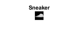
You can add a live control to your live script to explore your dataset:

i = 42;
img = reshape(train_images_m(i,:,:),[28,28]);
imshow(img)
title(class_names(tl(i)))
You must preprocess the data before training the network.
If you inspect the first image in the training set, you will see that the pixel values fall in the range of 0 to 255:
train_images = train_images / 255;
test_images = test_images / 255;
Finally, build and train the model with the function specified in the tf_helper file / module:
model = py.tf_helper.build_model();
You can look at the architecture of the model by retrieving the layers in a cell array:
cell(model.layers)
| 1 | 2 | 3 | |
|---|---|---|---|
| 1 | 1x1 Flatten | 1x1 Dense | 1x1 Dense |
py.tf_helper.compile_model(model);
py.tf_helper.train_model(model,train_images,train_labels)
Epoch 1/10

   1/1875 [..............................] - ETA: 12:59 - loss: 159.1949 - accuracy: 0.2500
  39/1875 [..............................] - ETA: 2s - loss: 52.8977 - accuracy: 0.5256
  76/1875 [>.............................] - ETA: 2s - loss: 34.8739 - accuracy: 0.6049
 113/1875 [>.............................] - ETA: 2s - loss: 28.4213 - accuracy: 0.6350
 157/1875 [=>............................] - ETA: 2s - loss: 22.9735 - accuracy: 0.6616
 194/1875 [==>...........................] - ETA: 2s - loss: 20.3405 - accuracy: 0.6740
 229/1875 [==>...........................] - ETA: 2s - loss: 18.3792 - accuracy: 0.6861
 265/1875 [===>..........................] - ETA: 2s - loss: 16.7848 - accuracy: 0.6943

 ...
Evaluate the model by comparing how the model performs on the test dataset:
test_tuple = py.tf_helper.evaluate_model(model,test_images,test_labels)
313/313 - 0s - loss: 0.5592 - accuracy: 0.8086 - 412ms/epoch - 1ms/step
test_tuple =
  Python tuple with values:

    (0.5592399835586548, 0.8086000084877014)

    Use string, double or cell function to convert to a MATLAB array.
test_acc = test_tuple{2}
test_acc = 0.8086
Test the model on the first image from the test dataset:
test_images_m = uint8(test_images);
prob = py.tf_helper.test_model(model,py.numpy.array(test_images_m(1,:,:)))
prob =
  Python ndarray:

    0.0000    0.0000    0.0000    0.0000    0.0000    0.0002    0.0000    0.0033    0.0000    0.9965

    Use details function to view the properties of the Python object.

    Use single function to convert to a MATLAB array.
[argvalue, argmax] = max(double(prob))
argvalue = 0.9965
argmax = 10
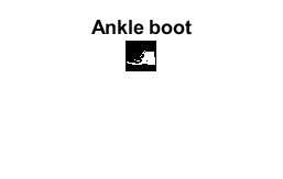
imshow(reshape(test_images_m(1,:,:),[28,28])*255)
title(class_names(argmax))
5.3. Import TensorFlow model into MATLAB
To illustrate the TensorFlow & ONNX import/export capabilities, we will take a workflow around an autonomous driving use case.

The data is generated by a simple open-source driving simulator from Udacity.
And the model comes from a real-life experiment from NVIDIA about End-to-end learning for self-driving cars.
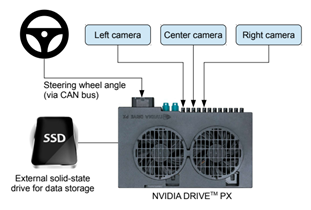
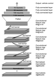
The inputs of the neural network are images from the camera and the output to predict in the steering angle (between -1 and 1).
We will simplify the problem with only 5 classes(from left to right).
(optional) Set up the parallel pool to use 4 workers for training on CPU
p = gcp('nocreate'); % If no pool, do not create new one.
if isempty(p)
   parpool()
else
    poolsize = p.NumWorkers
end
Import csv file created by the Udacity simulator with the images locations and the steering ground truth.
filename = "driving_log.csv";
drivinglog = import_driving_log( filename );
drivinglog = drivinglog(2:end,:)
| VarName1 | center | left | right | steering | throttle | reverse | speed | |
|---|---|---|---|---|---|---|---|---|
| 1 | 0 | “center_2021_04_25_1… | “left_202104_25_11… | “right_2021_04_25_11… | 0 | 0 | 0 | 0 |
| 2 | 1 | “center_2021_04_25_1… | “left_202104_25_11… | “right_2021_04_25_11… | 0 | 0 | 0 | 0 |
| 3 | 2 | “center_2021_04_25_1… | “left_202104_25_11… | “right_2021_04_25_11… | 0 | 0 | 0 | 0 |
| 4 | 3 | “center_2021_04_25_1… | “left_202104_25_11… | “right_2021_04_25_11… | 0 | 0 | 0 | 0 |
| 5 | 4 | “center_2021_04_25_1… | “left_202104_25_11… | “right_2021_04_25_11… | 0 | 0 | 0 | 0 |
Prepare data
Analyse the range of values for the steering angle to find the optimal class values.
figure;
histogram(drivinglog.steering);
title("Original steering angle distribution");
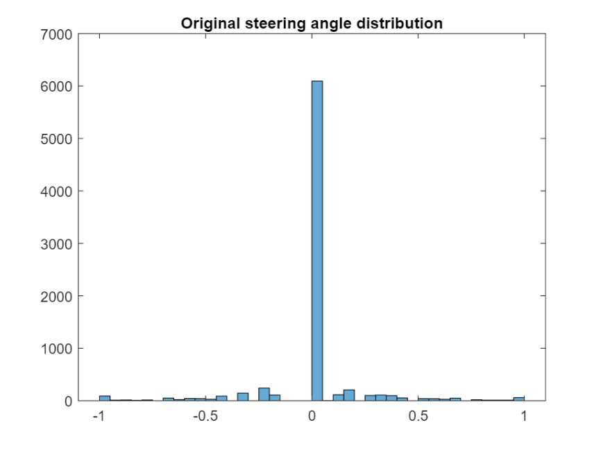
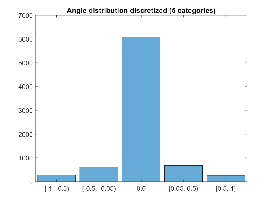
Use discretize to group the steering angles into discrete bins.
steeringLimits = [-1 -0.5 -0.05 0 0.05 0.5 1];
steeringClasses = discretize(drivinglog.steering, steeringLimits, 'categorical');
classNames = categories(steeringClasses);
Merge the two bins that represent the angle close to 0 degrees.
steeringClasses = mergecats(steeringClasses,["[-0.05, 0)","[0, 0.05)"], "0.0");
histogramClasses = histogram(steeringClasses);
title("Angle distribution discretized (5 categories)");
Create image datastore and balance data (undersampling)
The previous histogram shows that the dataset is highly unbalanced. Use countEachLabel to check how many instances there are of each class.
imds = imageDatastore("sim_data/"+drivinglog.center,"Labels", steeringClasses);
countEachLabel(imds)
| Label | Count | |
|---|---|---|
| 1 | [-1, -0.5) | 288 |
| 2 | [-0.5, -0.05) | 611 |
| 3 | 0 | 6093 |
| 4 | [0.05, 0.5) | 679 |
| 5 | [0.5,1] | 264 |
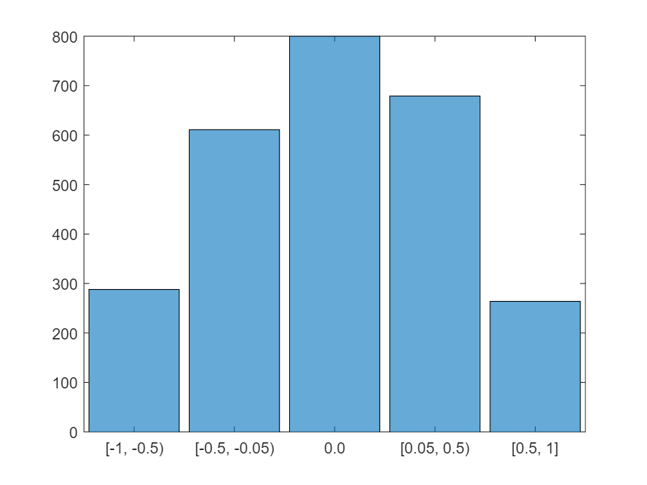
Define how many samples of the unbalanced class should be kept and randomly select these samples.
maxSamples = 800;
countLabel = countEachLabel(imds);
[~, unbalancedLabelIdx] = max(countLabel.Count);
unbalanced = imds.Labels == countLabel.Label(unbalancedLabelIdx);
idx = find(unbalanced);
randomIdx = randperm(numel(idx));
downsampled = idx(randomIdx(1:maxSamples));
retained = [find(~unbalanced) ; downsampled];
imds = subset(imds, retained');
histogram(imds.Labels)
Separate the dataset into training, validation and testing
Extract 90% of the data for training and the remaining for testing and validation.
[imdsTrain, imdsValid,imdsTest] = splitEachLabel(imds, 0.9, 0.05, 0.05);
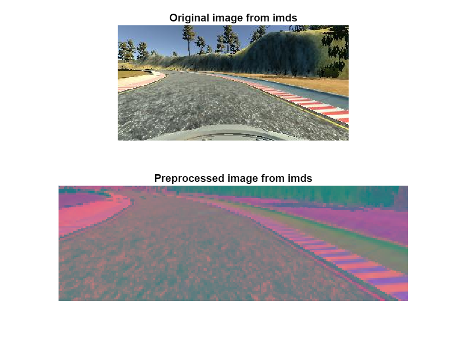
Preprocess the images by resizing it and converting it to the YCbCr color space.
trainData = transform(imdsTrain, @imagePreprocess, "IncludeInfo", true);
testData = transform(imdsTest, @imagePreprocess, "IncludeInfo", true);
valData = transform(imdsValid, @imagePreprocess, "IncludeInfo", true);
imds_origI = imdsTrain.read;
imds_newI = trainData.read{1};
subplot(211), imshow(imds_origI), title("Original image from imds")
subplot(212), imshow(imds_newI), title("Preprocessed image from imds")
Modify the model:
Load the network from keras model and display with Deep Network Designer.
It is recommended to save and import the model in the SavedModel format instead of the HDF5 format (you might get a warning).
layers = importKerasLayers("tf_model.h5")
layers =
  20x1 Layer array with layers:

     1   'conv2d_5_input'            Image Input         66x200x3 images
     2   'conv2d_5'                  2-D Convolution     24 5x5 convolutions with stride [2  2] and padding [0  0  0  0]
     3   'conv2d_5_elu'              ELU                 ELU with Alpha 1
     4   'conv2d_6'                  2-D Convolution     36 5x5 convolutions with stride [2  2] and padding [0  0  0  0]
     5   'conv2d_6_elu'              ELU                 ELU with Alpha 1
     6   'conv2d_7'                  2-D Convolution     48 5x5 convolutions with stride [2  2] and padding [0  0  0  0]
     7   'conv2d_7_elu'              ELU                 ELU with Alpha 1
     8   'conv2d_8'                  2-D Convolution     64 3x3 convolutions with stride [1  1] and padding [0  0  0  0]
     9   'conv2d_8_elu'              ELU                 ELU with Alpha 1
    10   'conv2d_9'                  2-D Convolution     64 3x3 convolutions with stride [1  1] and padding [0  0  0  0]
    11   'conv2d_9_elu'              ELU                 ELU with Alpha 1
    12   'flatten'                   Keras Flatten       Flatten activations into 1-D assuming C-style (row-major) order
    13   'dense'                     Fully Connected     100 fully connected layer
    14   'dense_elu'                 ELU                 ELU with Alpha 1
    15   'dense_1'                   Fully Connected     50 fully connected layer
    16   'dense_1_elu'               ELU                 ELU with Alpha 1
    17   'dense_2'                   Fully Connected     10 fully connected layer
    18   'dense_2_elu'               ELU                 ELU with Alpha 1
    19   'dense_3'                   Fully Connected     1 fully connected layer
    20   'RegressionLayer_dense_3'   Regression Output   mean-squared-error
deepNetworkDesigner(layers)
Remove the last layer used for regression and add the layers for a classification with 5 classes (then export net as layers_1)
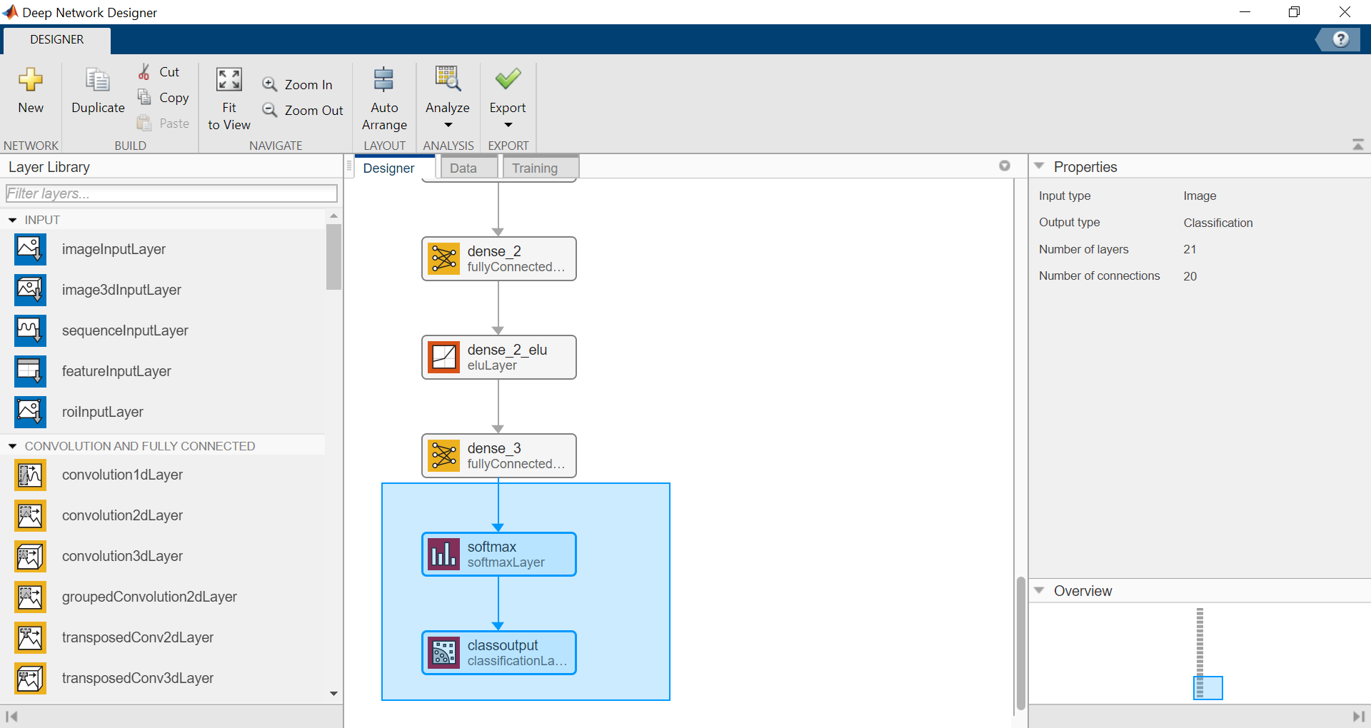
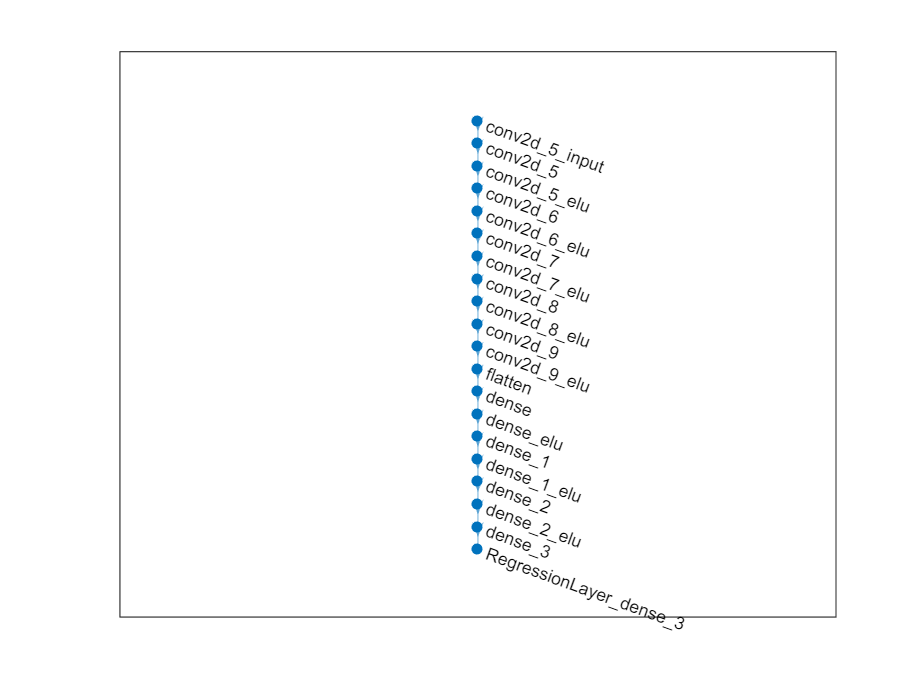
(programmatic alternative) Remove layers used for regression and add the layers for a classification with 5 classes
netGraph = layerGraph(layers);
clf; plot(netGraph)
classificationLayers = [fullyConnectedLayer(5,"Name","dense_3"), ...
                        softmaxLayer("Name","softmax"), ...
                        classificationLayer("Name","classoutput")];
netGraph = removeLayers(netGraph, {'dense_3', 'RegressionLayer_dense_3'});
netGraph = addLayers(netGraph,classificationLayers);
layers_1 = netGraph.Layers
layers_1 =
  21x1 Layer array with layers:

     1   'conv2d_5_input'   Image Input             66x200x3 images
     2   'conv2d_5'         2-D Convolution         24 5x5 convolutions with stride [2  2] and padding [0  0  0  0]
     3   'conv2d_5_elu'     ELU                     ELU with Alpha 1
     4   'conv2d_6'         2-D Convolution         36 5x5 convolutions with stride [2  2] and padding [0  0  0  0]
     5   'conv2d_6_elu'     ELU                     ELU with Alpha 1
     6   'conv2d_7'         2-D Convolution         48 5x5 convolutions with stride [2  2] and padding [0  0  0  0]
     7   'conv2d_7_elu'     ELU                     ELU with Alpha 1
     8   'conv2d_8'         2-D Convolution         64 3x3 convolutions with stride [1  1] and padding [0  0  0  0]
     9   'conv2d_8_elu'     ELU                     ELU with Alpha 1
    10   'conv2d_9'         2-D Convolution         64 3x3 convolutions with stride [1  1] and padding [0  0  0  0]
    11   'conv2d_9_elu'     ELU                     ELU with Alpha 1
    12   'flatten'          Keras Flatten           Flatten activations into 1-D assuming C-style (row-major) order
    13   'dense'            Fully Connected         100 fully connected layer
    14   'dense_elu'        ELU                     ELU with Alpha 1
    15   'dense_1'          Fully Connected         50 fully connected layer
    16   'dense_1_elu'      ELU                     ELU with Alpha 1
    17   'dense_2'          Fully Connected         10 fully connected layer
    18   'dense_2_elu'      ELU                     ELU with Alpha 1
    19   'dense_3'          Fully Connected         5 fully connected layer
    20   'softmax'          Softmax                 softmax
    21   'classoutput'      Classification Output   crossentropyex
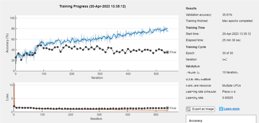
Train the model: (I am using my CPU here, but I recommend to speed it up on a GPU)
initialLearnRate = 0.001;
maxEpochs = 30;
miniBatchSize = 100;
options = trainingOptions("adam", ...
    "MaxEpochs",maxEpochs, ...
    "InitialLearnRate",initialLearnRate, ...
    "Plots","training-progress",  ...
    "ValidationData",valData, ...
    "ValidationFrequency",10, ...
    "LearnRateSchedule","piecewise", ...
    "LearnRateDropPeriod",10, ...
    "LearnRateDropFactor",0.5, ...
    "ExecutionEnvironment","parallel",...
    "Shuffle","every-epoch");
net = trainNetwork(trainData, layers_1, options);
Save model: Save the new trained network in a MAT format.
model_name = "net-class-30-1e-4-drop10-0_5"; % classification-epochs-learning_rate-drop_period-drop_factor
save(model_name+".mat","net")
Export it to a ONNXNetwork format.
exportONNXNetwork(net,model_name+".onnx")
Test model:
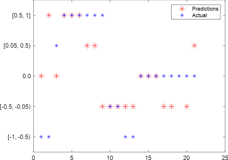
Plot predicted and ground truth values for steering angle using the testing dataset.
model_name = "net-class-30-1e-4-drop10-0_5"; % classification-epochs-learning_rate-drop_period-drop_factor
load(model_name+".mat","net")
predSteering = classify(net, testData);
figure
startTest = 80;
endTest = 100;
plot(predSteering(startTest:endTest), 'r*', "MarkerSize",10)
hold on
plot(imdsTest.Labels(startTest:endTest), 'b*')
legend("Predictions", "Actual")
hold off
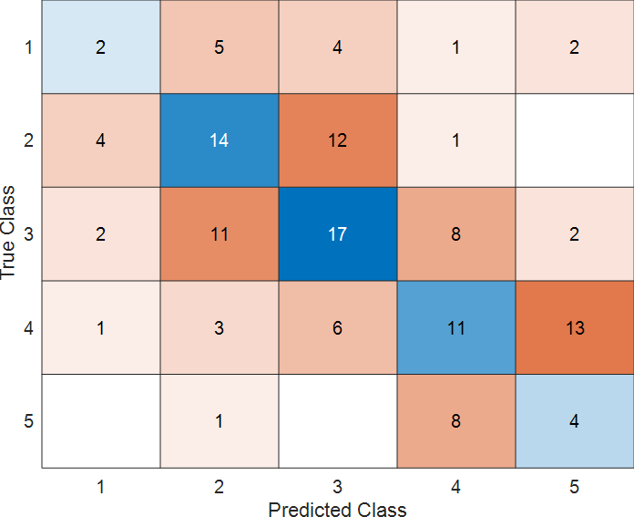
Display the confusion matrix.
confMat = confusionmat(imdsTest.Labels, predSteering);
confusionchart(confMat)
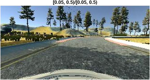
Display the testing image and the predicted label along with the ground truth.
numberImages = length(imdsTest.Labels);
i = 42;
img = readimage(imdsTest, i);
imshow(img),title(char(imdsTest.Labels(i)) + "/" +char(predSteering(i)));
Helper Functions
function drivinglog = import_driving_log(filename, dataLines)
%IMPORTFILE Import data from a text file
%  DRIVINGLOG = IMPORTFILE(FILENAME) reads data from text file FILENAME
%  for the default selection.  Returns the data as a table.
%
%  DRIVINGLOG = IMPORTFILE(FILE, DATALINES) reads data for the specified
%  row interval(s) of text file FILENAME. Specify DATALINES as a
%  positive scalar integer or a N-by-2 array of positive scalar integers
%  for dis-contiguous row intervals.
%
%  See also READTABLE.
%
% Auto-generated by MATLAB on 28-May-2021 21:31:34
%% Input handling
% If dataLines is not specified, define defaults
if nargin < 2
    dataLines = [1, Inf];
end
%% Set up the Import Options and import the data
opts = delimitedTextImportOptions("NumVariables", 8);
% Specify range and delimiter
opts.DataLines = dataLines;
opts.Delimiter = ",";
% Specify column names and types
opts.VariableNames = ["VarName1", "center", "left", "right", "steering", "throttle", "reverse", "speed"];
opts.VariableTypes = ["double", "string", "string", "string", "double", "double", "double", "double"];
% Specify file level properties
opts.ExtraColumnsRule = "ignore";
opts.EmptyLineRule = "read";
% Specify variable properties
opts = setvaropts(opts, ["center", "left", "right"], "WhitespaceRule", "preserve");
opts = setvaropts(opts, ["center", "left", "right"], "EmptyFieldRule", "auto");
opts = setvaropts(opts, ["VarName1", "steering", "throttle", "reverse", "speed"], "ThousandsSeparator", ",");
% Import the data
drivinglog = readtable(filename, opts);
end
function [dataOut, info] = imagePreprocess(dataIn, info)
imgOut = dataIn(60:135, :, :);
imgOut = rgb2ycbcr(imgOut);
imgOut = imresize(imgOut, [66 200]);
dataOut = {imgOut, info.Label};
end